Introduction

Electromagnetic geophysical exploration methods have been an open area of research since the 1950’s. The goal of such methods is to image the electrical properties of rock underground. Theoretically, deposits of minerals and hydrocarbons could be mapped in addition to voids like tunnels and mines. By measuring the electromagnetic fields at the surface of the earth the material properties of the rock underground can be inferred.

Since the earth is a relatively good conductor, VLF frequency techniques are preferred for their greater penetration depth. At 24kHz in the VLF band, the skin depth in Earth is approximately 100m, which would allow for greater imaging depths. By contrast, the penetration depth at higher frequencies used for ground penetrating radars is on the order of a few centimeters.

The classical far-field resolution of an image is restricted by the wavelength of imaging light, specifically the maximum spatial resolution is half the wavelength. However, the goal of this research project is to image on spatial scales far smaller than the far-field resolution limit. Such resolution can be achieved due to near-field interactions and the presence of evanescent mode waves near the surface [Cui et al. (2004)]. By recording near field evanescent modes at or near the surface of the earth, information about objects significantly smaller than the free space wavelength can be discerned and used for imaging.

The novelty of this project is to use ambient noise – namely signals from lightning or sferics – as a source. Every flash of lightning radiates the bulk of its radio frequency energy in the VLF band. Such signals propagate around the globe in the Earth-Ionosphere waveguide. Hundreds of sferics can be detected every minute. The waveform of a sferic is relatively short in the time domain, yielding a richer content in the frequency domain. Furthermore, this project focuses on looking at subsurface imaging in complex topographies, or mountainous regions. Such flexibility increases the complexity of the inversion methods necessary.

This project has thus far consisted of two components, data collection and data inversion.

Data Collection

Field Work

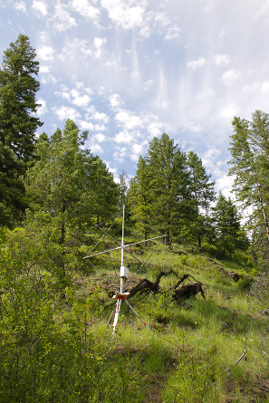
For this project, three orthogonal components of the magnetic field are recorded with a set of Stanford VLF Group AWESOME receivers [Cohen et al. (2010)]. The receiver was modified to fit in a waterproof case and to run autonomously on battery power. Timing synchronization of 20ns between receivers is achieved using GPS. Each receiver has a unique phase and amplitude calibration to remove bias. A wireless link can be used in the field to maintain contact with each of the receivers deployed, although recent improvements in the recording software have made the individual receivers more robust decreasing the need for such a link. Sets of 12, 5, 3, and 2 receivers have been used for campaigns in Alaska, Arizona, Colorado, Idaho, Kansas, and Nevada. The antenna, as deployed in Idaho can be seen in Figure 1.

**Figure 1:**
Three axis magnetic field antenna deployed in Northern Idaho. July, 2010

Sferics

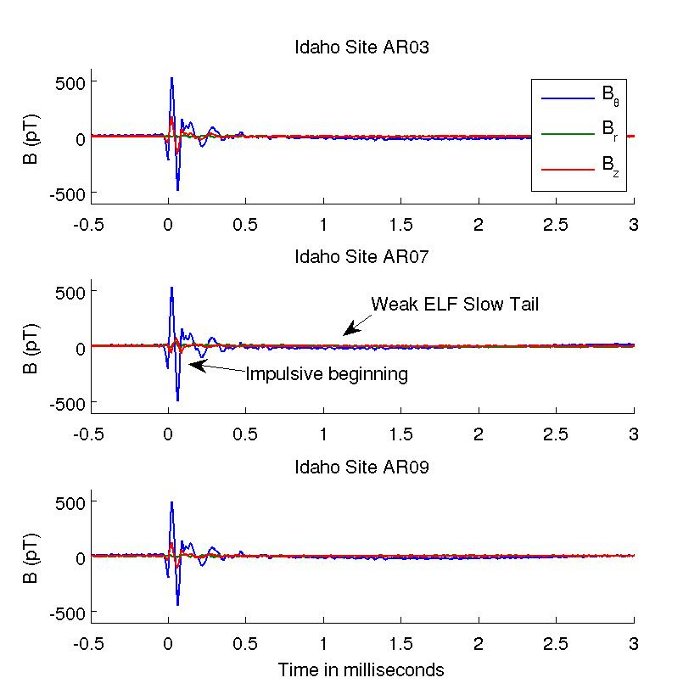
In the field, hundreds of sferics are recorded each minute. They are easily identified in the data and can be correlated with national and global lightning detection databases to identify the location and propagation path of each sferic. An example of a sferic recorded in Idaho is shown in Figure 2. Since sferics propagate predominantly in a transverse magnetic mode, the magnetic field orthogonal to the surface of the earth () can be a proxy indicator of anomalous material properties.

**Figure 2:**
Example of sferics recorded in Northern Idaho, August, 2009.. “ $B_\theta$ ” is the magnetic field perpendicular to the direction of propagation, “” is parallel to the direction of propagation, and is the direction normal to the flat earth.

Inverse Problem

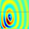
The electromagnetic methods for geophysical imaging are typically cast as an optimization problem. Given a model of electromagnetic wave propagation, perturbations to the model can be introduced and optimized so as to match the data predicted by the model to the data actually recorded as illustrated in Figure 3. This inverse problem, determining the scattering materials from scattered wave measurements, is ill-posed and has been the subject of much activity [Abubakar et al. (2009)]. The sophistication and detail of the model significantly affects the computational time necessary for inversion. Two methods have so far been investigated, a 1D layered earth model, and a 2D finite difference frequency domain (FDFD) model.

**Figure 3:**
The goal of the inverse problem is to determine the value of the anomalous conductivity and permittivity buried in a conductive half-space.

1D model

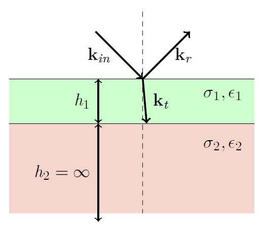
Assuming that a sferic can be approximated as a plane-wave in a transverse magnetic (TM) waveguide mode, interactions with the earth can be modeled with reflection and transmission coefficients. Reflection coefficients for an arbitrary number of layers composed of linear media are given by Wait (1970).

With a simple two layer model that can be rotated to arbitrary angles to conform to the local topography, surprisingly good matches can be made between an assumed incident wave and the data recorded. This result suggests that a large constituent of the anomalous signal can be explained by surface reflection effects. Such a model, while useful for a first order approximation of the surface conductivity, is limited in scope, resolution, and accuracy.

**Figure 4:**
Model for layered medium. The reflection coefficient can be calculated exactly by knowing the electrical properties and dimensions of the subsurface layers.

FDFD based model

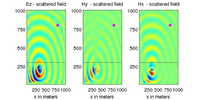
As suggested by Dong and Rappaport (2009), finite difference frequency domain methods can be used as a basis for inversion. By invoking the Born approximation, a linearized algorithm for reconstructing the scattering materials can be formulated from knowledge of the background and scattered fields (Figure 5). Such an approach can provide fast, but resolution and contrast limited results. These methods and more accurate, iterative methods are currently under development.

**Figure 5:**
Scattered fields calculated in a conductive half space. A conductivity and permittivity anomaly is is outlined by the white box. Pink box indicates the location of a electric dipole point source.

Bibliography

Abubakar, A., T. M. Habashy, M. Li, and J. Liu (2009), Inversion algorithms for large-scale geophysical electromagnetic measurements, Inverse Problems, 25(12), 123,012.
Cohen, M., U. Inan, and E. Paschal (2010), Sensitive broadband ELF/VLF radio reception with the AWESOME instrument, IEEE Transactions on Geoscience and Remote Sensing, 48(1), 3-17.
Cui, T., W. Chew, X. Yin, and W. Hong (2004), Study of resolution and super resolution in electromagnetic imaging for half-space problems, IEEE Transactions on Antennas and Propagation, 52(6).
Dong, Q., and C. Rappaport (2009), Microwave subsurface imaging using direct finite-difference frequency-domain-based inversion, IEEE Transactions on Geoscience and Remote Sensing, 47(11).
Wait, J. R. (1970), Electromagnetic Waves in Statified Media, Pergamon Press.